Abstract
In this paper, a classification of three classes of medical devices manufactured by Stening® was carried out. The classification was performed using three machine learning algorithms oriented to classification. The algorithms were Support Vector Machines, Logistic Regression and Decision Tree. With this study, Stening® aims to make its products better known and to provide a more technical view of them.
Introduction
The main objectives of the study are the following:
- to make known the products that Stening® manufactures
- to offer a more technical view of them using innovative technology
In this work, a classification of three classes of medical devices manufactured by Stening® was carried out. For this, three different machine learning classification techniques were used. These are three algorithms that do the same thing but whose internal workings are completely different. They were: Support Vector Machine (SVM), Logistic Regression (LG) and Decision Tree (DT). The internal workings will be explained in the theoretical foundation.
- ST (Tracheal Stent)
- TM (T-tube)
- SY (Stent in "Y")
Three datasets of 900, 1200 and 1500 rows were generated to perform the training. For the classification we relied on 5 different but common attributes of the devices: length, diameter, anchors, number of branches and wall thickness. These 5 attributes are what differentiate, within the dataset, the three classes of medical device. The creation of the dataset will be explained in the results section.
We will analyze the results of each algorithm applied to each of the datasets. Finally, the conclusions and future outlook of this study will be given.
Type of study
This is a computational study oriented to the field of artificial intelligence.
Theoretical foundation
In this section we will introduce the algorithms used for the classification of the medical devices.
SVM
In this section the Support Vector Machines algorithm [1] will be introduced. It is a classification algorithm belonging to the branch of supervised learning. It performs the classification by finding the best hyperplane1 in an N-dimensional space (N being the number of parameters) that separates the data.
To separate two classes of data there are many possible hyperplanes. The goal of the algorithm is to find the one that is at the greatest distance between the data of both classes (see figure 1).
The hyperplanes mark the zone where one class begins and another ends. That is, if in the future we receive a parameter in the lower zone of the hyperplane it will be of the red class; if it is in the other zone it will be blue. The hyperplanes can be of different dimensions, depending on the data we have. If we have a dataset {x1, x2}, as in figure 1, our hyperplane will be a straight line; if the data depend on three different attributes {x1, x2, x3} the hyperplane will be of dimension two. In other words, it will always have one dimension less than our dataset.
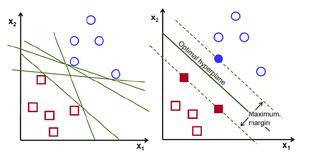
Figure 1: hyperplane for 2D [2].
The support vectors are data points close to the hyperplane that influence its orientation and positioning. In SVM we seek to maximize the margin between the points and the hyperplane.
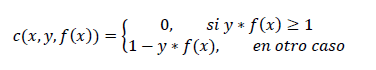
The function that will help us maximize the margin is the following:
(1)
Expression (1) is called the loss function. In this expression, x is the data, y is the known result and f(x) is the prediction we make. If these last two have the same sign, the loss function equals zero.
This algorithm is used for classification problems and for making predictions. For example, distinguishing between three types of flowers from three different data points: x = {color, petal width, height}. Then, after learning from the data, the model must be able to predict which class of flower (y) a flower with data it has not seen belongs to.
Logistic Regression
Logistic regression is a statistical method for performing classifications [3]. It is a special type of linear regression where the classes to be predicted are categorical. This can be understood with an example: predicting whether I have a disease or not, the answers would be Yes or No.
As stated, it is a special type of linear regression. The formula of a linear regression is the following:
(2)
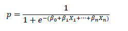
In expression (2), y is the result of the prediction and X1, X2, ... are the variables with which the model trains. We obtain logistic regression by introducing (2) into the following expression:
(3)
Expression (3) is called the Sigmoid function (figure 2). So, logistic regression consists of applying the sigmoid function to a linear regression.
We have three types of logistic regression:
- Binary logistic regression: two categories to predict
- Multinomial logistic regression: three or more categories to predict
- Ordinal logistic regression: three or more categories to predict, but ordinal, that is, with a certain order
In this work we will use multinomial logistic regression, since we have three classes of medical devices; it will not be ordinal because they lack order.
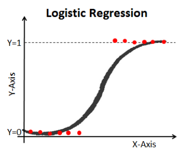
Figure 2: Graphical representation of a binary logistic regression [3].
Decision Tree
A decision tree is a widely used algorithm, not only in Machine Learning but in other areas of computing [4]. Its logic is simpler than that of the other two algorithms, since it is more intuitive. We will explain this logic below.
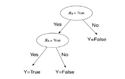
The decision tree has three main components: nodes, leaves and branches. A node represents an attribute, a branch represents a decision and a leaf represents an output. The main objective is to generate a decision tree that has as many leaves as the categories you want to classify, in our case three, since we have three different types of medical device. The structure would be like that of figure 3.
Results
In this section we will explain how we built the dataset and the results obtained.
Dataset
We built the dataset from the measurements of the original Stening® devices. Three different datasets of 900, 1200 and 1500 rows each were created.
As stated, from the dimensions of the devices manufactured by Stening®, we generated the datasets randomly. This gave us training freedom to have greater variety. This is so because some dimensions included on its website are not the best-selling and therefore the least manufactured, so if we relied on that to generate the dataset, even though it would be closer to reality it would bias the model and the training. That is why, as a first approximation, we decided to generate the dataset in this way. Nevertheless, as stated, always within the real dimensions of the devices.
In the following image we can see a series of rows of the 1200 dataset:
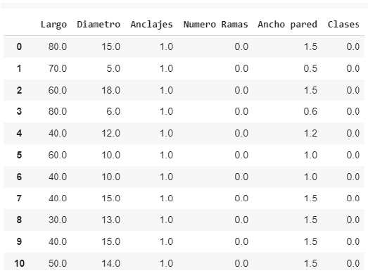
Figure 4: First 11 rows of the 1200-row dataset.
As there are 3 different classes of device, a number was assigned to each in order to train the models. In this way: '0' represents an ST, '1' a TM and '2' an SY. In turn, for the binary parameters (Yes/No) such as the column ("Anchors"), a '1' was assigned if the answer was 'Yes' and a '0' if the answer was 'No'.
A program written in Python 3.5 was used to build the dataset.
Programs and results
Three programs were made, one for each model to be applied. Each of the three datasets was fed into these three programs, thus obtaining three results per algorithm. These three programs were written, like the one that generates the dataset, in Python 3.5. The machine learning library Sklearn was used to make them.
As for the results obtained, absolute efficacy was obtained in the three models. Each of them was able to obtain 100% efficacy in predicting samples it had not seen before. In the following images we can see the results obtained:
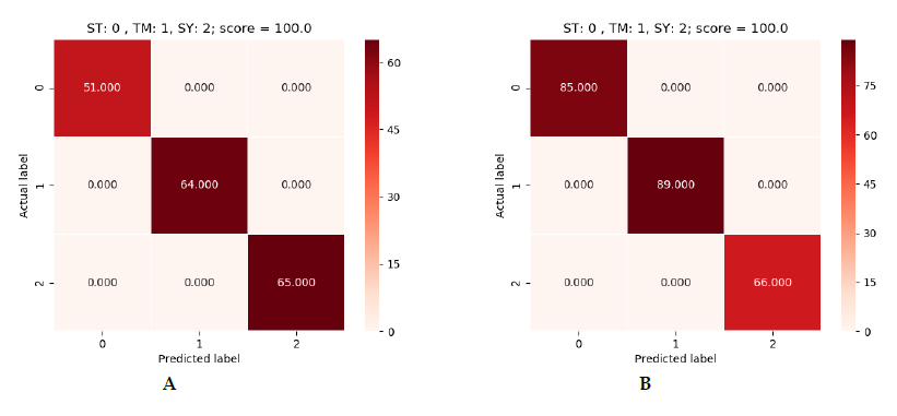
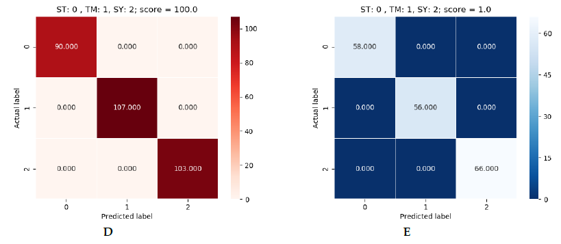
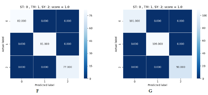
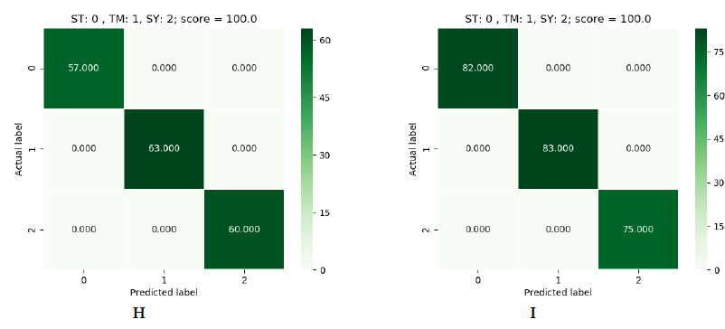
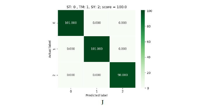
Figure 5: green (SVM), blue (Logistic Regression) and red (Decision Tree).
In figure 5 we can see the results obtained for each dataset. As stated, there are three result tables per algorithm. They are in order, the first being the 900 one and the last the 1500 one. In each table we can see a reference to the labels. On the vertical axis we have the correct label and on the horizontal axis the label predicted by the model. In the upper-right corner we have the prediction result. The number that appears inside the square is the number of devices predicted with that label. If we add up all the numbers we will see that the total of the dataset is not obtained, since these are the predictions on a part of the dataset that the model did not see during training. This is because the dataset was divided into 70% for training and 30% for making predictions.
Conclusions
To conclude, it is worth mentioning that the results obtained are very satisfactory. This motivates us to continue investigating and carrying out studies related to machine learning and artificial intelligence.
Footnotes
- It is a plane of dimension N-1, N being the total dimension of the space we are in (1D, 2D, 3D...)
References
- Support Vector Machine, https://towardsdatascience.com/support-vector-machine-introduction-to-machine-learning-algorithms-934a444fca47
- Support Vector Machine, https://towardsdatascience.com/support-vector-machine-introduction-to-machine-learning-algorithms-934a444fca47 Fig. 1
- Logistic Regression, https://www.datacamp.com/community/tutorials/understanding-logistic-regression-python
- Decision Tree, https://medium.com/deep-math-machine-learning-ai/chapter-4-decision-trees-algorithms-b93975f7a1f1
- Decision Tree, https://hackernoon.com/what-is-a-decision-tree-in-machine-learning-15ce51dc445d.